
Originally published with the IFRS 17 Discount Rate Working Party in 2021.
This paper looks at the practical issues with developing a credit model in the calculation of the IFRS 17 discount rate. A recent paper(henceforth known as “the Educational Note”) by the Canadian Institute of Actuaries [1] includes a discussion of various credit models and this paper looks at one particular application of the Through-The-Cycle (TTC) type model. One of the models referenced in the Educational Note is an implementation of the Vasicek model [2], and this model is investigated in this paper. There are many possible credit models that could be used and no model is endorsed, but we show some of the issues by investigating this particular model referenced in the Educational note.
The IFRS 17 discount rate calculation is presented and the role of the credit model in the IFRS 17 discount rate is given. The credit model mentioned in the Educational Note is described together with some sources for data that can be used to calibrate it. Some of the advantages and key limitations of this model are described. Finally, a paragraph-by-paragraph summary comparing the TTC model with the IFRS 17standards.
The calculation of the IFRS 17 discount rate requires one of two approaches:
· The top-down approach - Calculate the yield on assets backing liabilities and subtract a default allowance; with the default allowance calculated from a credit model
· The bottom-up approach - Calculate the “risk free” rate and add on a liquidity premium
Some firms have applied a third hybrid type approach where a default allowance is calculated on the assets backing the liabilities (in line with the top-down approach). This is removed from the yield on these assets to give a liquidity premium, which is then added to the “risk free” rate(in line with the bottom-up approach). This hybrid approach is similar to the Solvency II Matching Adjustment style calculation. The main two (non-hybrid)approaches are shown below:
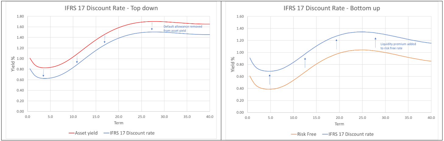
Figure 1 – Bottom-up and top-down approaches to IFRS 17 discount rate calculation
In section 3 of this paper, a credit model is described in some detail including a description of transition matrices in section 3.1. Section 3.2 describes different sources of unexpected default risk and section 3.3 describes the Belkin model. Section 3.4 comments on possible data sources and 3.5 gives a practical example of the credit model including results and sensitivities. Section 4 includes a comparison with how the credit model described in this paper compares to the IFRS 17 standards.
This paper focuses on the calculation of the default allowance which is required whether a top-down approach or a hybrid approach are used (as described above). This paper does not consider how to calculate a liquidity premium directly (other than by calculating the default allowance and subtracting from the credit spread). This paper does not endorse a hybrid or top-down approach – but only shows some of the issues with such approaches. To quantify the default allowance a credit model is required. The credit model considered in this paper is as referenced in the Educational Note[3]. The credit model for the IFRS 17 default allowance is required to include both expected and unexpected defaults[4]. The Educational Note described two possible credit models that allow for expected and unexpected defaults; a Point In Time(PIT) approach and a Through The Cycle (TTC) approach.
In this paper we focus on the TTC approach and show the considerations for applying it in practice; how it meets the IFRS 17 standard as well as issues and limitations. The model considered is known as the Belkin implementation of the Vasicek model (henceforth known as the Belkin model). The model uses historical transition matrices to calibrate the Vasicek model.
We start be giving a brief overview of transition matrices and how these are used to calculate expected defaults. We then consider different ways to allow for unexpected defaults. There is then a review of the Belkin model and possible sources of data that can be used to calibrate it.
Transition matrices are used to present historical probabilities of moving between different credit ratings and defaults. They are constructed by counting the number of corporate bonds that have moved credit rating or defaulted over a particular time period.
An example from S&P is shown below which captures the one-year transition and default probabilities calculated based on averages over the period 1981-2018.
From this transition matrix the probability of going from AAA to AA is 9.42% over a one-year time period. The probability of a B rated asset defaulting over a one-year time period is 3.93%.
One of the strengths of the transition matrix is the simplicity with which probabilities at other terms can be found. Using Markov assumptions, we can simply multiply a one-year transition probability matrix by itself to get the two-year transition probabilities. For example, the above matrix multiplied by itself gives the two-year probability of transitioning between ratings or defaults.
Two-year transition probabilities (based on 1981-2018 data).
The probability of a B rated asset defaulting over a two-year time period is 8.92%.
In principle we can use this approach to calculate default probabilities over any time frame. This is the approach use to calculate“ expected defaults”, which give the best estimate without any margin for unexpected defaults.
The credit model should include an allowance for unexpected defaults over and above the best estimate. For a credit risk there are two potential sources of unexpected defaults:
· An unexpected credit event
· Mis-estimation of long term expected defaults
These are shown graphically in the plot below:
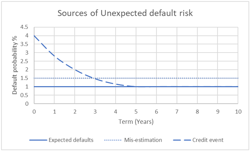
The plot above shows representative example for two sources of unexpected default risk.
· An unexpected credit event is an event where credit defaults are higher than has been seen on average historically (e.g.1932 or the 2008 financial crisis). This event might last a number of years as is shown in the plot above. The unexpected event does not need to be an extreme event as might be required for capital calculations, but some margin needs to be allowed for to cover unexpected defaults
· Mis-estimation of long term expected defaults is the risk that the estimate of the expected defaults is too low.
A TTC model for the IFRS 17 discount rate credit model could include one or both of these elements to cover the firm’s view of how much reserves it needs to hold for unexpected defaults. The exact allowance for unexpected defaults is not specified in the IFRS 17 standards.
The Belkin Model is well described in a note by JP Morgan [5] which includes a precise description of its calibration using historical transition matrices. There is also amore recent article in The Actuary magazine [6] describing some of the historical context and practical issues associated with this model.
The main strength of this model is its simplicity and ease of explanation as each transition matrix is represented by a single number. In principle this number represents whether the year was a good or bad year and by what magnitude, for transitions and defaults. Once the model has been calibrated, transition matrices at different percentiles can be generated, which could be used to allow for the unexpected default risk.
The main limitation of the model is precisely that it represents an entire transition matrix with just a single number inevitably this results in a loss of information. It is possible to measure the volatility of each rating in each transition matrix and these vary considerably across the different ratings. It is possible to use the market value of assets actually held as weightings for each rating in the calibration of the Belkin model to create a weighted average.
Another limitation is that the model uses the Normal distribution to model credit risk. At the high percentiles this is not a good representation of the underlying risk which is typically fat tailed (and skewed). This is shown in the plot below:
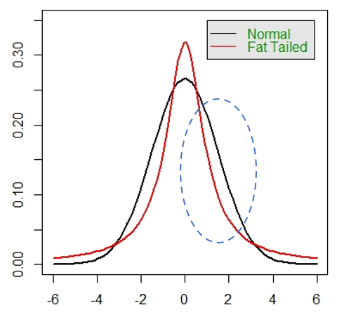
However, the IFRS 17credit model is a model for best estimate plus a margin for unexpected defaults and the percentile used is likely to be in the range where the Normal is above a fatter tailed distribution (i.e., the range highlighted with a blue circle above), on this basis this limitation is not expected to understate the risk, as it would where an extreme percentile is being considered.
Users of this model need to ensure they are familiar with the model limitations and how these limitations impact the use to which the model is being put.
This section gives a summary of the main data sources used for transition matrices.
It is possible to find S&P transition matrix data online (without charge) back to 1981 (with the exception of a few years). However, the main data source of historical transition matrices (requires a subscription) is the Moody’s data source which includes annual transition matrices from 1920-2019. A plot showing historical transition matrices calibrated to the Belkin model is shown below[7].
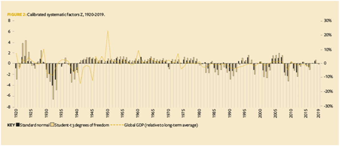
This plot shows the Z score values for each historical transition matrix back to 1920. The black bars are from a standardised Normal distribution (grey bars from using a fatter tailed standardised Student T distribution). The left scale in the plot above shows how many standard deviations from the mean each historical transition matrix is represented by (e.g. 1932 is just under 4 standard deviations from the mean using the Normal distribution Belkin model as described in that article). (Right axes in the above plot relates to change in Global GDP and not directly relevant to this paper.)
This plot gives a full range of historical data to calibrate a model to including:
· The 1930s Great depression
· The “Golden era” from 1945-1970 of economic growth
· The 2008-09 Great financial crisis
This section gives a simple example calibration for illustrative purposes. In practice, significantly more rigour wouldbe expected for a default allowance calibration.
The Belkin model described in the previous section has been calibrated to the freely available data source described in section 3.4 as well as a year of extreme stress [8] (i.e. years 1932, 1981-2003, 2006-2018).
For unexpected defaults a simple approach was used and in practice significantly more justification would be required. This simple approach was to use:
· No weighting between the different rating in the calibration of the Belkin model
· The 95th percentile for the long-term mis-estimation risk
· No allowance for a short-term unexpected credit event(see section 3.2)
· 30% recovery rate
Using this version of the model, default allowance can be calculated as a probability, which can then be converted to a spread.
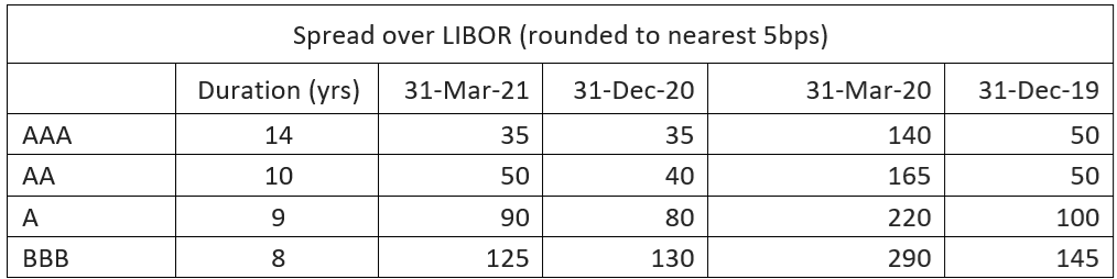
Some credit spreads for various ratings and durations during recent periods together with the Covid stress as at March 31 2020 are shown below.
The expected default allowance as a percentage of these credit spreads is shown in the table below:
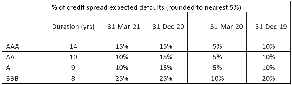
The expected defaults shown in the above table allows for all the possible ways a bond could move between ratings to default over the duration. For example, the 15% shown in the top left cell is the probability of default for a AAA rated bond over 14 years moving over any possible rating over that period and ending in default. (This calculation is done using the multiplication of transition matrices as described in section 3.1, which captures the movement between ratings and ending in default at or before 14 years.)
The expected and unexpected default allowance as a percentage of these credit spreads is shown in the table below:
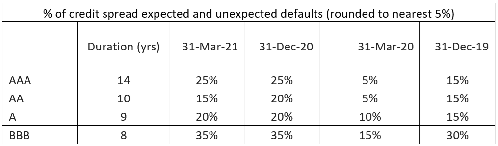
Note that these results hold for as a percentage over swaps, but the results would be different if gilt rates were used as the risk free.
The results for 31 March 2020 show that when credit spreads are much higher (as was the case at this point in the covid crisis) the default allowance takes a significantly lower proportion of credit spreads (i.e. default allowance remains stable, but is a lower proportion of a higher credit spread).
In this section we include a sensitivity on the final table in the previous section, showing the impact of a higher recovery rate of 40% (all other assumptions the same).

We also include a sensitivity with the 80th percentile (instead of 95th) all other assumptions unchanged (i.e. recovery at 30%).
% of credit spread expected and unexpected defaults (rounded to nearest 5%)
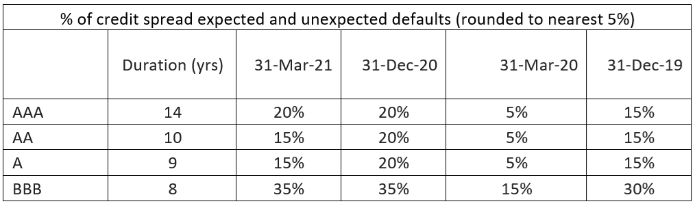
The exact percentile used is a subjective choice, which has some dependence on the firms view of how risk averse investors are with respect to unexpected credit risk.
This section shows an interpretation for how a TTC model meets the IFRS 17 standards.
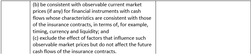
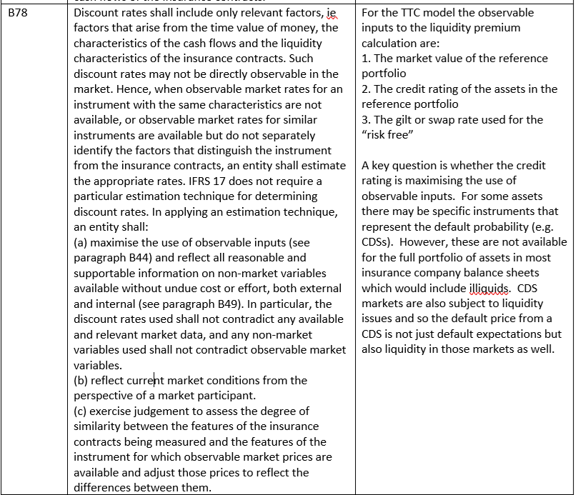
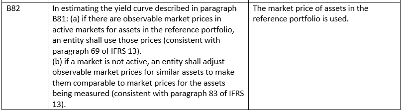
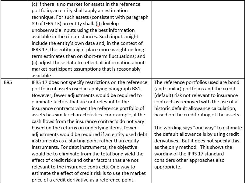
Discount rates are covered in Paragraphs 36and B72 – B85 of the IFRS 17 standard. Specific points that apply to the default allowance for discount rates are given in paragraphs 36, B78, B82, B83, B85. These are shown in the table below, together with a justification for how the TTC approach meets the standard.
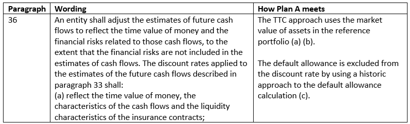
In this paper, the IFRS 17 discount rate calculation is presented and the role of the credit model in the IFRS 17 discount rate is given. The credit model mentioned in the Educational Note is described together with some sources for data that can be used to calibrate it. Some of the advantages and key limitations of this model are described. Finally, a paragraph-by-paragraph summary is given for why a TTC model is in line with the IFRS 17 standards.
[1] “IFRS 17 Discount Rates for Life and Health Insurance Contracts” Canadian Institute of Actuaries [https://www.cia-ica.ca/publications/publication-details/220079]
[2] “A one-parameter representation of credit risk and transition matrices” D Belkin, L Forest 1998 [https://www.z-riskengine.com/media/1032/a-one-parameter-representation-of-credit-risk-and-transition-matrices.pdf]
[3] “A one-parameter representation of credit risk and transition matrices” D Belkin, L Forest 1998 [https://www.z-riskengine.com/media/1032/a-one-parameter-representation-of-credit-risk-and-transition-matrices.pdf]
[4] See Canadian Institute of Actuaries Educational note: “IFRS 17 Discount Rates for Life and Health Insurance Contracts” June 2020 P26 section 4.2.2
[5] “A one-parameter representation of credit risk and transition matrices” Belkin B, Suchower S [a-one-parameter-representation-of-credit-risk-and-transition-matrices.pdf(z-riskengine.com)]
[6] “Glide rule: credit migration and default risk” | The Actuary Ginghina F, Kapadia A [https://www.theactuary.com/features/2021/02/26/glide-rule-credit-migration-and-default-risk]
[7] “Glide rule: credit migration and default risk” | The Actuary Ginghina F, Kapadia A [https://www.theactuary.com/features/2021/02/26/glide-rule-credit-migration-and-default-risk]
[8] 1932 year from [https://www.bundesbank.de/resource/blob/635454/3d26f24706559d386b04a2efd06d5d7c/mL/2011-10-19-eltville-11-varotto-paper-data.pdf];remaining years sourced from Extreme Events Working Party
