
Published with kind permission of www.insuranceerm.com. Original article April 2016: https://www.insuranceerm.com/analysis/optimising-hypothecation-in-matching-adjustment-portfolios.html
The matching adjustment (MA) is a provision under Solvency II designed to help insurers with long-term liabilities – in particular, UK annuity providers –meet the solvency capital requirement.
The regulation values assets and liabilities on a mark-to-market basis, meaning that valuations can fluctuate day-by-day. For an insurer that typically buys long-duration fixed income assets with the intention of holding them for the duration, short-term volatility is of little concern. But the market movements can make their solvency position look bad and could potentially force them to dispose of assets at fire-sale prices.
The MA is an addition to the risk-free rate used to discount annuitant liabilities and its main benefit is a significant reduction in the size of these liabilities. Its use requires regulatory approval and the UK’s Prudential Regulation Authority (PRA) has so far allowed 16 firms to benefit.
The MA is intended to represent the part of the credit spread associated with the lower liquidity of assets relative to assets earning the risk-free rate. The part of the credit spread associated with the risk of default or downgrade is called the fundamental spread.
The fundamental spread is calculated monthly by the European Insurance and Occupational Pensions Authority (EIOPA). This has been subject to several revisions, but is now expected to be relatively stable. This means that as credit spreads move, the matching adjustment and credit spreads are expected to move quite closely and so reduce balance sheet volatility.
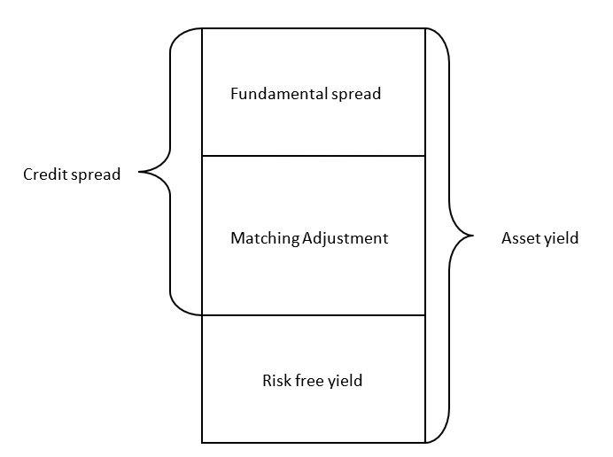
Figure 1 –the matching adjustment relative to other components of the asset yield.
Where, fundamental spread = max(x% LTAS, P(default) + CostDowngrade)
LTAS= Long Term Average Spread
X%= 30% or 35% depending on the asset type
Some firms are looking to reapply for the MA to optimise the benefit they gain and others will be seeking to apply for the first time. The process of creating an optimal MA has typically involved selecting assets with the highest MA to go into the MA portfolio (assets with a higher MA are typically less liquid and higher yielding). This is only part of the challenge, with a further issue in the hypothecation process required to select the subset of assets in the MA portfolio on which the MA itself is based. By careful selection, significant gains in MA benefit can be achieved – as discussed below.
The MA is calculated for an MA portfolio - which is a ring-fenced fund of liabilities closely matched with assets. This ring-fenced fund contains enough assets to cover the Best Estimate Liabilities (BEL) plus a small surplus. EIOPA and the PRA have set out how the MA is to be calculated in Solvency II regulations and in a number of PRA letters. A summary of how this calculation has been prescribed is below:
Removing the last part of the fundamental spread from the component A assets means that the market value of the component A assets is less than the BEL. The additional assets required to meet the BEL are the component B assets and the assets in surplus above BEL are the component C assets. Components A, B and C were defined as such by the PRA. The largest proportion of the MA portfolio is typically the component A assets (e.g. 80-95%). A small surplus (the component C assets) is usually held in the MA portfolio which might be up to 5%, but potentially significantly less than this.
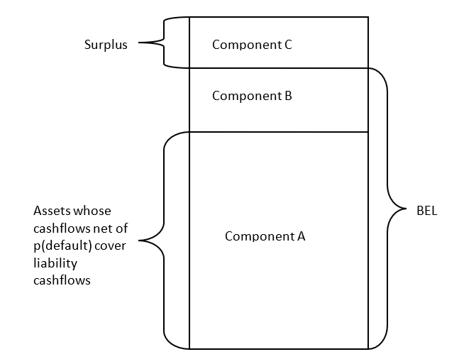
Figure 2 – showing the split of MA portfolio into asset components A, B and C
As well as the steps above, the component A and B assets are required to pass three matching tests set out by the PRA. These tests are:
As the MA value is dependent on just component A assets, how these are selected is material. For example, a firm could go to the effort of acquiring high-yielding assets with good MA, only to find that the team doing the hypothecation do not include these assets in component A, and they are left in component B or C.
There are three potential ways of doing the hypothecation:
1. By hand – going through each asset and setting a percentage between 0%-100% for how much is in component A and B, whilst ensuring the PRA tests are met and the MA is as high as possible;
2. Automated matching – automating the by-hand method using an algorithm that goes through each term matching assets to liabilities, with a tendency to choose assets of higher MA in component A; or
3. Using a numerical method to optimise the MA whilst keeping within the PRA tests.
Neither the PRA nor EIOPA have specified any approach to the hypothecation, so in this area there is full choice about how to best maximise the MA.
Doing the hypothecation by hand has the main advantage that it has more limited set up costs. However, the downsides are significant in that it:
Using an automated matching approach will reduce the time spent doing the hypothecation, but it will not remove the other two disadvantages of the by-hand approach.
The alternative is to use a numerical method for the hypothecation. Relative to the other approaches, this will
The numerical method approach works with two key steps:
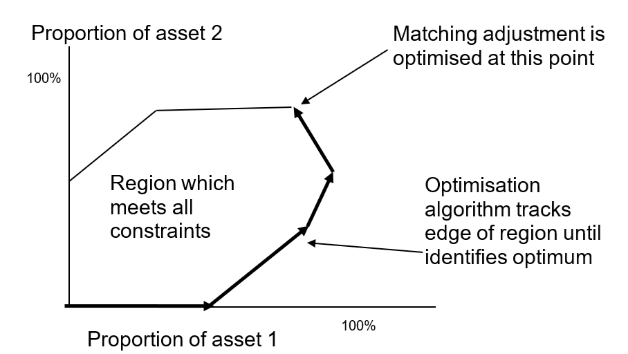
The first step involves careful consideration of the constraints imposed on the hypothecation amounts by the MA calculation itself, as well as the constraints imposed by the three PRA matching tests. Once a region of possible hypothecations has been identified which meets the PRA tests and the MA calculation requirements, the next step is to identify which hypothecation will give the highest MA.
The region which meets all the required constraints is a multi dimensional shape – with as many dimensions as there are assets in the MA portfolio. There are a variety of numerical methods which can be used to solve this problem; some of which skirt around the outside of this shape until they find the optimum, whilst others will go through the interior of this shape. The main thing is to have a numerical method which finds the optimum solution in as short as possible time.
Relative to hypothecating by hand it may be that the MA can be increased by 10-15 basis points by optimising the hypothecation. For many firms this will be a significant reduction in liabilities and well worth getting right.
This article has set out that an important part of optimising the MA lies within the MA calculation process itself. Whilst other aspects of optimising the MA are important, the hypothecation step should not be ignored and a very small initial investment can lead to extremely large reductions in liabilities as well as process improvements.
It is possible that in the upcoming Solvency II reviews that the scope of the MA is extended, which may make this process of hypothecation even more important.
James Sharpe is a director of actuarial consultancy Sharpe Actuarial Limited. Email: james@sharpeactuarial.co.uk
